How Node Enumeration Turns Actuarial Guesswork into Computation
Context. Parts 1–8 defined the coverage node and the NodeID receipt: a node is drug × indication × clinical criteria (CNID) × plan overlay (POID) × commercial terms (COID), and a NodeID is a verifiable hash of those documents plus scope. This part shows how enumerated nodes enable actuarial underwriting and multi‑contract RFPs with math that is simple, auditable, and tractable at scale.
1) Why actuarial precision needs nodes
Trend‑based pharmacy underwriting averages across members, benefits, and hidden rebates. It cannot price rule‑level risk. Node enumeration exposes the real contractable variables:
- Eligibility logic (CNID): explicit rules that decide who qualifies, when, and why.
- Operational overlay (POID): channel/site‑of‑care, accumulator stance, dispense limits, dividend policy.
- Commercial terms (COID): flat nets (fixed net per 30‑day equivalent), fixed‑gain admin fee, optional outcomes escrow.
When rules and nets are explicit, population risk becomes a sum over members and nodes, not a trend guess.
2) The ingestion figure — why it’s clever
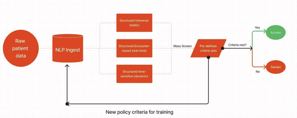
Your intake model splits reality into three streams:
- Structured Universal (static): demographics, chronic diagnoses, historical contraindications
- Structured Encounter‑based (real‑time): new orders, diagnoses, and labs as they arrive
- Structured Time‑sensitive (dynamic): pregnancy, acute windows, temporary exclusions
All three feed a mass screen → pre‑defined criteria sets step. If a member meets a CNID’s rules, the claim adjudicates at the published flat net (Yes → Access). If not, it routes to Denied or human review. A feedback loop promotes edge‑cases into new policy criteria, so the catalog improves without retraining the world.
3) Notation and objects
- Members: P\mathcal{P}P. Months t=1,…,Tt=1,\dots,Tt=1,…,T.
- Nodes: N\mathcal{N}N. Each node j∈Nj\in\mathcal{N}j∈N has CNID CjC_jCj, POID PjP_jPj, COID KjK_jKj, and scope.
- Flat net price: netj\text{net}_jnetj (USD per 30‑day equivalent).
- Restrictiveness: ρj∈[0,1]\rho_j\in[0,1]ρj∈[0,1] (0=open; 1=most restrictive). A simple monotone schedule:

- (More open criteria → lower flat net; more restrictive → higher. You’re pricing volume/risk explicitly—the transparent analogue to “bigger rebate for open access.”)
Deterministic eligibility
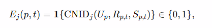
where UpU_pUp (Universal), Rp,tR_{p,t}Rp,t (Encounter), and Sp,tS_{p,t}Sp,t (Time‑sensitive) are the three intake layers.
Uptake probability: uj(p,t)∈[0,1]u_j(p,t)\in[0,1]uj(p,t)∈[0,1] (grows as member sees the real net and friction falls).
Adherence share (PDC proxy): aj(p,t)∈[0,1]a_j(p,t)\in[0,1]aj(p,t)∈[0,1] (falls with member cost + friction).
📊 Claims, RFPs & Contracting — Let’s Run the Numbers
Need a quick claims evaluation, an RFP scoring narrative, or help pressure‑testing contract terms, pricing, or actuarial assumptions? Hit the button — your email will open pre‑filled with options.
✉️ Request Ops/Analytics Support- Claims eval: denial drivers & PA friction by policy language
- RFP prep: variance storylines + scoring narrative
- Contract review: rebate & guarantee terms, transparency language
- Pricing/GTN scenarios: sensitivity & risk bounds
- Actuarial forecast: trend, mix, & unit-cost drivers
4) Population accounting — series you can measure
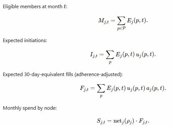
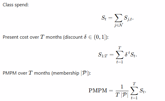
These are the core sums over sets. They’re computable with this pipeline and verifiable with NodeID receipts.
5) Outcomes escrow you can underwrite
Let the metric be “PDC ≥ 80% at 6 months.” For members on node jjj, with indicators Yp∈{0,1}Y_p\in\{0,1\}Yp∈{0,1} and MjM_jMj evaluable members:
- Observed rate: O^j=1Mj∑Yp\hat{O}_j = \frac{1}{M_j}\sum Y_pO^j=Mj1∑Yp.
- One‑sided lower confidence bound (illustrative, Wald):
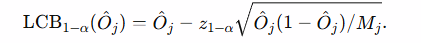
Pick a target τ\tauτ. Size escrow EjE_jEj so the ex ante risk to both sides is neutral: refund EjE_jEj to payer if LCB1−α(O^j)<τ\text{LCB}_{1-\alpha}(\hat{O}_j) < \tauLCB1−α(O^j)<τ; otherwise release to manufacturer. The COID fixes the oracle (data sources, censoring, window).
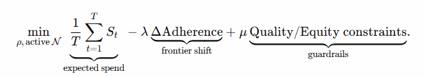
6) Optimization views
Plan objective (choose criteria ρ\rhoρ and active nodes):
Manufacturer objective (pick net,ρ\text{net},\rhonet,ρ on a frontier):
Π=(net−c)∑tFt−EscrowRisk\Pi = (\text{net}-c)\sum_t F_{t} – \text{EscrowRisk}Π=(net−c)∑tFt−EscrowRisk
subject to volume FFF and elasticity. Negotiation reduces to pairs (ρ,net(ρ))(\rho,\text{net}(\rho))(ρ,net(ρ)) on a shared frontier.
7) RFP kit — running multi‑contract bids with nodes
Include in the RFP packet:
- CNID ladder (A/B/C) per class (human‑readable + JSON).
- COID menu: flat nets, fixed‑gain fee, optional outcomes escrow (oracle spec baked in).
- POID overlay: channel/site‑of‑care, accumulator stance, dividend policy.
- KPI deck: NPA, Friction Minutes, Price–Adherence Frontier, Outcomes Yield (definitions + formulas).
- Verification: NodeID receipt spec + sample signed receipts.
Bid format (per rung): submit net(ρ)\text{net}(\rho)net(ρ) and (if used) escrow schedule E(ρ)E(\rho)E(ρ), plus readiness and explicit cohort exclusions.
Ops: sandbox adjudication → go‑live; weekly NodeID receipt extracts (no PHI) for audit; quarterly ladder reviews (any change = new NodeID, old receipts remain verifiable).
8) Messaging the economics — “flat nets” and restrictiveness
- Use flat nets everywhere: the number at the counter equals the plan net.
- Treat restrictiveness ρ\rhoρ as a slider: open (ρ → 0\rho\!\to\!0ρ→0) → lower net but higher eligibility; restrictive (ρ → 1\rho\!\to\!1ρ→1) → higher net and lower eligibility. Total spend is the observable result of both.
- This mirrors today’s rebate logic (open access ↔ bigger rebate) minus the opacity: we quote flat nets directly.
Bottom line: Enumerated nodes convert pharmacy underwriting from trend‑based guesswork into auditable sums over explicit rules. That’s what payers can buy, what manufacturers can price, and what patients can verify at the counter.
Savings math
If baseline pharmacy PMPM = BBB, current YoY trend = rrr, and you can land a lower trend r′r’r′ via node‑based design, annual savings across NNN members is: Annual savings=12×N×B×(r−r′).\text{Annual savings} = 12 \times N \times B \times (r – r’).Annual savings=12×N×B×(r−r′).
Example (100k lives; r = 10.7%, r’ = 7.0%; Δ = 3.7 percentage points):
| Baseline PMPM BBB | Savings PMPM =B×0.037= B \times 0.037=B×0.037 | Annual Savings @ 100k lives |
|---|---|---|
| $150 | $5.55 | $6.66M |
| $250 | $9.25 | $11.10M |
| $400 | $14.80 | $17.76M |